Author: Ed Nelson
Department of Sociology M/S SS97
California State University, Fresno
Fresno, CA 93740
Email: ednelson@csufresno.edu
Note to the Instructor: The data set used in this exercise is gss14_subset_for_classes_STATISTICS_pspp.sav which is a subset of the 2014 General Social Survey. Some of the variables in the GSS have been recoded to make them easier to use and some new variables have been created. The data have been weighted according to the instructions from the National Opinion Research Center. This exercise uses CROSSTABS in PSPP to explore crosstabulation. I prepared two documents to help you with PSPP – “Notes on Using PSPP” and “Differences between PSPP and SPSS” which should answer many of your questions about PSPP. You have permission to use this exercise and to revise it to fit your needs. Please send a copy of any revision to the author. Included with this exercise (as separate files) are more detailed notes to the instructors and the PSPP syntax necessary to carry out the exercise. Please contact the author for additional information.
I’m attaching the following files.
- Data subset (.sav format)
- Extended notes for instructors (MS Word; docx format).
- PSPP syntax file (.sps format)
- This page (MS Word; docx format).
Goals of Exercise
The goal of this exercise is to introduce crosstabulation as a statistical tool to explore relationships between variables. The exercise also gives you practice in using CROSSTABS in PSPP.
Part I—Relationships between Variables
In exercises STAT5S through STAT8S we used sample means to analyze relationships between variables. For example, we compared men and women to see if they differed in the number of years of school completed and the number of hours they worked in the previous week and discovered that men and women had about the same amount of education but that men worked more hours than women. We were able to compute means because years of school completed and hours worked are both ratio level variables. The mean assumes interval or ratio level measurement (see STAT2S_pspp).
But what if we wanted to explore relationships between variables that weren’t interval or ratio? Crosstabulation can be used to look at the relationship between nominal and ordinal variables. Let’s compare men and women (d5_sex) in terms of the following:
- opinion about abortion (a1_abany),
- fear of crime (c1_fear),
- satisfaction with current financial situation (f4_satfin),
- opinion about gun control (g1_gunlaw),
- gun ownership (g2_owngun),
- voting (p5_pres08), and
- religiosity (r8_reliten).
Before we look at the relationship between sex and these other variables, we need to talk about independent and dependent variables. The dependent variable is whatever you are trying to explain. In our case, that would be how people feel about abortion, fear of crime, gun control and ownership, voting and religiosity. The independent variable is some variable that you think might help you explain why some people think abortion should be legal and others think it shouldn’t be legal or any of the other variables in our list above. In our case, that would be sex. Normally we put the dependent variable in the row and the independent variable in the column. We’ll follow that convention in this exercise.
Let’s start with the first two variables in our list. We’re going to use a1_abany as our measure of opinion about abortion. Respondents were asked if they thought abortion ought to be legal for any reason. And we’re going to use c1_fear as our measure of fear of crime. Respondents were asked if they were afraid to walk alone at night in their neighborhood. Run CROSSTABS in PSPP to produce two tables. One will be for the relationship between d5_sex and a1_abany. The other will be for d5_sex and c1_fear. Put the independent variable in the column and the dependent variable in the row. By default PSPP will give you the counts as well as the row, column, and total percents. In this case you want only the counts and column percents. That means you will want to uncheck the boxes for the row and total percents so you won’t have unnecessary and perhaps confusing numbers in your output.
PSPP will list the variables and you will select those variables you want to use. PSPP lists the variables using the variable labels. However, it’s easier to find the variables if they are listed by variable names. You can change the way PSPP lists the variables by right clicking anywhere on the list of variables and selecting “Prefer variable labels” and that will list the variables by name. However, you will have to do this each time you encounter a list of variables. There is no way to do this permanently.
Your instructor will probably talk about how to compute these different percents. But how do you know which percents to ask for? Here’s a simple rule for computing percents.
- If your independent variable is in the column, then you want to use the column percents.
- If your independent variable is in the row, then you want to use the row percents.
Since you put the independent variable in the column, you want the column percents.
Part II – Interpreting the Percents
Your first table should look like this.
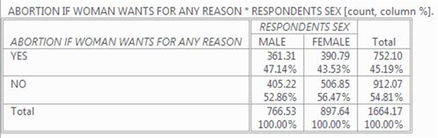
It’s easy to make sure that you have the correct percents. You independent variable (d5_sex) should be in the column and it is. Column percents should sum down to 100% and they do.
How are you going to interpret these percents? Here’s a simple rule for interpreting percents.
- If your percents sum down to 100%, then compare the percents across.
- If your percents sum across to 100%, then compare the percents down.
Since the percents sum down to 100%, you want to compare across.
Look at the first row. Approximately 47% of men think abortion should be legal for any reason compared to 44% of women. There’s a difference of 3.61% which is really small. We never want to make too much of small differences. Why not? No sample is ever a perfect representation of the population from which the sample is drawn. This is because every sample contains some amount of sampling error. Sampling error in inevitable. There is always some amount of sampling error present in every sample. The larger the sample size, the less the sampling error and the smaller the sample size, the more the sampling error. So in this case we would conclude that there probably isn’t any difference in the population between men and women in their approval of abortion for any reason.
Now let’s look at your second table.
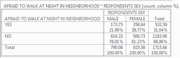
This time the percent difference is quite a bit larger. About 22% of men are afraid to walk alone at night in their neighborhood compared to 39% of women. This is a difference of 16.78%. This is a much larger difference and we have reason to think that women are more fearful of being a victim of crime than men.
Part III – Now it’s Your Turn
Choose two of the tables from the following list and compare men and women:
- satisfaction with current financial situation (f4_satfin),
- opinion about gun control (g1_gunlaw),
- voting (p5_pres08), and
- religiosity (r8_reliten).
Make sure that you put the independent variable in the column and the dependent variable in the row. Be sure to ask for the correct percents. What are values of the percents that you want to compare? What is the percent difference? Does it look to you that there is much of a difference between men and women in the variables you chose?
Part IV – Adding another Variable into the Analysis
So far we have only looked at variables two at a time. Often we want to add other variables into the analysis. Let’s focus on the difference between men and women (d5_sex) in terms of gun ownership (g2_owngun). First let’s get the two-variable table which should look like this.
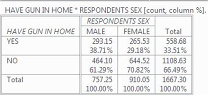
Men were more likely to own guns by 9.53%. But what if we wanted to include social class in this analysis? The 2014 GSS asked respondents whether they thought of themselves as lower, working, middle, or upper class. This is variable d11_class. What we want to do is to hold constant perceived social class. In other words, we want to divide our sample into four groups with each group consisting of one of these four classes and then look at the relationship between d5_sex and g2_owngun separately for each of these four groups. Social class will be our control variable since we are going to hold it constant.
In order to run a table with a control variable, we need to create a blank syntax file. To do this click on “File” in the menu bar and then on “New” and finally on “Syntax.” A blank syntax file should open. Enter the following commands into the syntax file. It’s easiest to do this by copying and pasting the commands into the syntax file.
CROSSTABS
/TABLES=g2_owngun BY d5_sex BY d11_class
/STATISTICS=CHISQ GAMMA
/CELLS=COUNT COLUMN.
To run this commands click on “Run” in the menu bar and then on “All.” You should see the following table in your output window.
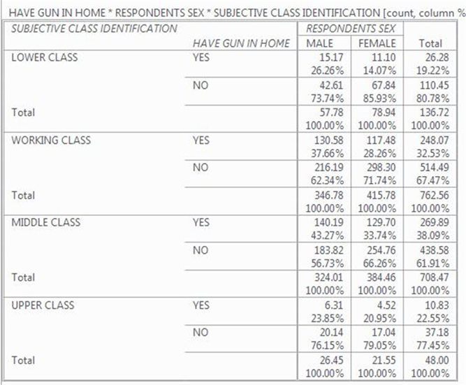
This table is more complicated. Notice that the table is actually divided into four tables with one on top of the other. At the top we have those who said they were lower class, then working, middle and upper class. Let’s look at the percent differences for each of these tables – 12.19%, 9.40%, 9.53%, and 2.90%. The first three tables are similar to the two-variable table – 9.53% compared to 11.19%, 9.40%, and 9.53%. Remember not to make too much out of small differences because of sampling error. Notice that the last table for upper class has a much smaller difference – 2.90%. In other words, when we look at only those who see themselves as upper class, there really isn’t any difference between men and women in terms of gun ownership.
But notice something else. There are fewer people who say they are lower and upper class than say they are working or middle class. There are only 137 respondents in the lower class table and even fewer, 48 respondents, in the upper class table. We’ll have more to say about this in the next exercise (STAT10S).
Part V – Now it’s Your Turn Again
In Part II we compared men and women (d5_sex) in terms of fear of crime (c1_fear). Run this table again but this time add social class (d11_class) into the analysis as a control variable as we did in Part IV. What happens to the percent difference when you hold constant class? What does this tell you?
Recall from Part IV that to run a table with a control variable, we need to create a blank syntax file. To do this click on “File” in the menu bar and then on “New” and finally on “Syntax.” A blank syntax file should open. Enter the following commands into the syntax file. It’s easiest to do this by copying and pasting the commands into the syntax file.
CROSSTABS
/TABLES=c1_fear BY d5_sex BY d11_class
/STATISTICS=CHISQ GAMMA
/CELLS=COUNT COLUMN.
The only difference between this and what you did in Part IV is that you have substituted c1_fear for g2_owngun.

