Chapter 5: Correlation

Chapter
5 examines the relationship between pairs of variables. Correlation and regression
are both statistical techniques for doing this, and in this chapter we focus
on some examples of correlation; Chapter 6 examines simple regression techniques.
Correlation measures the strength of a linear relationship and determines whether
it is positive or negative. Is an increase in disposable income associated with
an increase in consumption? Is an increase in economic growth associated with
a fall in the unemployment rate (Okun’s Law)? Is a fall in the unemployment
rate associated with a rise in inflation (Phillips curve)? Measures of correlation
indicate whether changes in the value of one variable is associated with changes
in the value of another.

Correlation does
not tell us anything about causation. In fact, some variables move together
due to randomness, or because they are both caused by something else. For
example, the number of police in a community is correlated with the crime
rate and, I’ve been told, the number of teachers in a given population is
correlated with rates of alcoholism. The naive researcher incorrectly concludes
that (1) police cause crime, and (2) teachers cause alcoholism. In the first
case, the direction of causation is probably from crime to police, not vice
versa. In the second case, the association of the two variables is due to
pure chance (I hope). In no case do measures of correlation tell us about
causation. For that, we must rely on some form of social theory (e.g., economics
or sociology or political science, etc.) to explain association.

5-1
Visualizing correlation I: consumption and income

It is helpful to
have notation for correlation. Define the correlation measure for two populations
as r (the Greek letter rho) and the sample measure as r. The formula for the
sample correlation of variables X and Y is:

Sample correlation
= r_XY = [Covariance of (X,Y)] / Ö (s_Xs_Y),

where s_X
and s_Y are the standard deviations of X and Y.

The value of
the correlation coefficient, r, must lie between -1 and 1:

1 ³ r ³
-1.

Correlation coefficients
of minus one and one imply that X and Y are perfectly correlated. Minus one
indicates a perfect negative correlation (X up, Y down), and +1 a perfect
positive correlation (X up, Y up). Any variables that are perfectly correlated
are measuring the same thing, for example degrees centigrade and degrees Fahrenheit,
or dollars and pesos. Every degree centigrade equals 9/5 degrees Fahrenheit,
and every dollar equals (about) 8 Mexican pesos. Temperature and money values
can be measured using different scales, but in the final analysis, its the
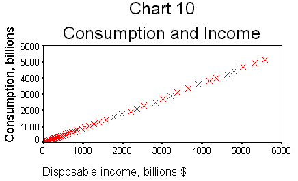
same thing.

Consider the
relationship between consumption and disposable income. Economists have known
for several decades that these two variables are associated with each other.
If fact, they have about as close an association as possible without being
perfectly correlated. Let's use SPSS to construct the scatter plot of the
two variables consumption (c in the dataset) and disposable personal income
(dp1).

1. Choose
   Graphs from the menu bar, then select Scatter . . .;
2. Make sure
   the Simple box is selected, and then click Define;
3. Highlight
   c in the variable list box and use the arrow to move it to the Y Axis
   box;
4. Do the
   same for dp1 and move it into the X Axis box;
5. Click OK.

After editing, your
graph should look like Chart 10.

 

Note the close
relationship between the two; they practically lie on a straight line with
a positive slope. Now, calculate the correlation coefficient:

1. Choose
   Statistics from the menu bar, then select Correlate;
2. Select
   Bivariate . . .;
3. Highlight
   c in the variable list box and move it into the Variables box;
4. Do the
   same for dp1, and click OK.

SPSS puts correlation
coefficients, r, in a matrix. The diagonal elements are the correlation of a
variable with itself (it must be 1.00), and the off-diagonals are the correlation
of the row and column variables. Due to symmetry, you really only need to look
at the top triangular part of the matrix. Each entry has 3 numbers, the correlation
coefficient, the number of observations in parentheses, and the p-value, which
is a measure of the statistical significance of the correlation coefficient.

Consumption and
disposable personal income are as correlated as two variables can be without
being the same thing (0.9998). There are 68 observations, and the p-value
is zero to the nearest 4 decimal places. The p-value is actually a statistical
test: H₀: r = 0, H₁: r¹ 0.

The p-value is
the probability of observing the actual sample outcome (r = 0.9998) if the
null hypothesis (H₀: r = 0) is true. The usual procedure is to
reject the null hypothesis if the p-value is less than 0.05 (meaning we have
less than a 5% chance of getting our data if the null hypothesis is true;
better to reject the null hypothesis if we observe something rare.)

5-2
Visualizing correlation II: inflation, wages, unemployment and the deficit

Let's compare this
result to others where the correlation is not so strong. In each of the following,
we create a graph and the correlation. You will see that as the scatter plot
points disintegrate from a straight line into a random jumble, the correlation
statistic gets closer to zero.

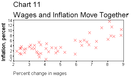
Inflation
and wages

Consider first the
relationship between wages and inflation. In an earlier exercise we computed
inflation as the percentage change in the CPI, inflation = p = [(cpi - lag(cpi))/lag(cpi)]
* 100.

If you have not
done this yet, use the Transform, Compute functions in SPSS to do it now.
We use inflation in the following exercises. Also, calculate the percentage
change in average hourly earnings (ahe) in the same way.

The question
is whether wages keep up with inflation. When inflation rises, does the nominal
wage too? If so, then the purchasing power of wages stays constant, which
is to say that real wages do not change. Chart 11 shows this
relationship.

 

Calculate the
correlation coefficient. Are changes in wages and prices perfectly correlated?
How correlated are they?

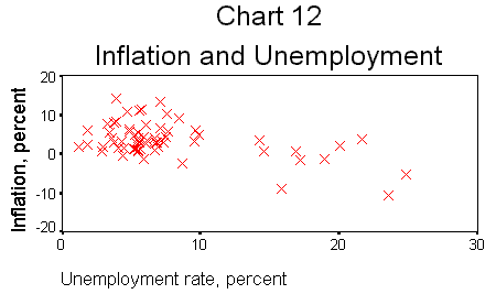
Inflation
and unemployment

The Phillips curve
is the scatter plot relationship between inflation and unemployment. Chart
12 plots these variables.

 

Note that the
scatter plot shows a predominantly negative relationship whereas the other
two (inflation/wages, and consumption/income) were positive. Calculate the
correlation between inflation and unemployment and note that it is negative.
Is inflation more or less correlated with unemployment than it is with changes
in wages? Can you see the difference in the tightness of the scatter in Charts
10, 11, and 12?

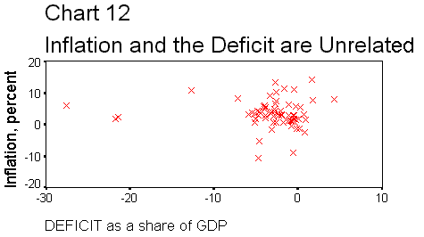
Inflation
and the deficit

Let’s tell a story
about the economy that relates inflation to the federal budget deficit. When
the government runs a deficit, it injects new purchases into the economy which
are greater than what it takes out with taxes. This increases total spending
(aggregate demand) and causes shortages of some goods because spending is greater
than production. Firms respond by raising prices and we get inflation. So, deficits
cause inflation. If we compute the correlation statistic, it should show a significant
positive relationship. That is, we expect to find r > 0, and to reject the null
hypothesis, H₀: r = 0.

Chart 13
is the scatter plot between inflation and a new variable which we computed
as (deficit/gdp). (We computed this new variable last chapter; do so now if
you have not done it yet).

 

It is the deficit,
measured as a percentage of GDP.) The correlation statistic turns out to be
-0.0383. This is the wrong sign, and the p-value says that there is a high
probability of observing this correlation if the null hypothesis is true.
We reject the null hypothesis. It looks like we have to either tell a different
story, or probe deeper for a connection between inflation and deficits. The
latter may not uncover anything, but it definitely requires more statistics.