STAT15S_SDA - Exercise Using SDA to Explore Multiple Linear Regression

Author:   Ed Nelson
Department of Sociology M/S SS97
California State University, Fresno
Fresno, CA 93740
Email:  ednelson@csufresno.edu

Note to the Instructor: This exercise uses the 2014 General Social Survey (GSS) and SDA to explore multiple linear regression.  SDA (Survey Documentation and Analysis) is an online statistical package written by the Survey Methods Program at UC Berkeley and is available without cost wherever one has an internet connection.  The 2014 Cumulative Data File (1972 to 2014) is also available without cost by clicking here.  For this exercise we will only be using the 2014 General Social Survey.  A weight variable is automatically applied to the data set so it better represents the population from which the sample was selected.  You have permission to use this exercise and to revise it to fit your needs.  Please send a copy of any revision to the author. Included with this exercise (as separate files) are more detailed notes to the instructors and the exercise itself.  Please contact the author for additional information.

I’m attaching the following files.

• Extended notes for instructors (MS Word; .docx format).
• This page (MS Word; .docx format).

I’m attaching the following files.

Goals of Exercise

The goal of this exercise is to introduce multiple linear regression.  The exercise also gives you practice using REGRESSION in SDA.

Part I – Linear Regression with Multiple Independent Variables

We’re going to use the General Social Survey (GSS) for this exercise.  The GSS is a national probability sample of adults in the United States conducted by the National Opinion Research Center (NORC).  The GSS started in 1972 and has been an annual or biannual survey ever since. For this exercise we’re going to use the 2014 GSS.  To access the GSS cumulative data file in SDA format click here.  The cumulative data file contains all the data from each GSS survey conducted from 1972 through 2014.  We want to use only the data that was collected in 2014.  To select out the 2014 data, enter year(2014) in the Selection Filter(s) box.  Your screen should look like Figure 15_1.  This tells SDA to select out the 2014 data from the cumulative file.

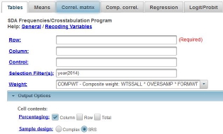
Figure 15-1

Notice that a weight variable has already been entered in the WEIGHT box.  This will weight the data so the sample better represents the population from which the sample was selected.  Notice also that in the SAMPLE DESIGN line SRS has been selected.

The GSS is an example of a social survey.  The investigators selected a sample from the population of all adults in the United States.  This particular survey was conducted in 2014 and is a relatively large sample of approximately 2,500 adults.  In a survey we ask respondents questions and use their answers as data for our analysis.  The answers to these questions are used as measures of various concepts.  In the language of survey research these measures are typically referred to as variables.  Often we want to describe respondents in terms of social characteristics such as marital status, education, and age.  These are all variables in the GSS.

In the previous exercise (STAT14S_SDA) we considered linear regression for one independent and one dependent variable which is often referred to as bivariate linear regression.  Multiple linear regression expands the analysis to include multiple independent variables.  In the first part of this exercise we’re going to focus on two independent variables.  Then we’re going to add a third independent variable into the analysis.  An important assumption is that “the dependent variable is seen as a linear function of more than one independent variable.”  (Colin Lewis-Beck and Michael Lewis-Beck, Applied Regression – An Introduction, Sage Publications, 2015, p. 55)

In the last exercise (STAT14S_SDA) we used tvhours as our dependent variable which refers to the number of hours that the respondent watches television per day.  In other words, we wanted to understand why some people watch more television than others.  We found that age was positively related to television viewing and father’s education was negatively related.  Older respondents tended to watch more television and respondents whose fathers had more education tended to watch less television. 

Let’s start by using FREQUENCIES in SDA to get the frequency distribution for tvhours.  In the previous exercise (STAT14S_SDA) we discussed outliers and noted that there are a few individuals (i.e., 14) who watch a lot of television which we defined as 14 or more hours per day.  We also noted that outliers can affect our statistical analysis so we decided to remove these outliers from our analysis. 

Let’s exclude these individuals by selecting out only those cases for which tvhours is less than 14. That way the outliners will be excluded from the analysis. To do this add tvhours(0-13) to the SELECTION FILTER(S) box.  Be sure to separate year(2014) and tvhours(0-13) with a space or a comma.  This will tell SDA to select out only those cases for which year is equal to 2014 and tvhours is less than 14.  Run FREQUENCIES in SDA to get a frequency distribution for tvhours after eliminating the outliers and check to make sure that there are no values greater than 13.

In bivariate linear regression we have one independent and one dependent variable.  So we are trying to find the straight line that best fits the data points in a two-dimensional space.  With two independent and one dependent variable we have a three-dimensional space.  So now we’re trying to find the plane that best fits the data points in this three-dimensional space. 

With two independent variables our regression equation for predicting Y is a + B₁X₁ + B₂X₂ where a is the constant, B₁ and B₂ are the unstandardized multiple regression coefficients, and X₁ and X₂ are the independent variables.  As with bivariate linear regression we want to minimize error where error is the difference between the observed values and the predicted values based on our regression equation.  It turns out that minimizing the sum of the error terms doesn’t work since positive error will cancel out negative error so we minimize the sum of the squared error terms.[1]  

Part II – Getting the Regression Coefficients

The regression equation will contain the values of a, B₁, and B₂ that minimize the sum of the squared errors.  There are formulas for computing these coefficients but usually we leave it to SDA to carry out the calculations.

Click on REGRESSION at the top of the SDA page and enter your dependent variable (tvhours) in the DEPENDENT box.  In the previous exercise (STAT14S_SDA) we ran two bivariate linear regressions – one with tvhours and age and a second with tvhours and paeduc.  In this exercise we’re going to use both independent variables simultaneously.  Enter both age and paeduc in the INDEPENDENT BOX so they become your independent variables.  Make sure that the WEIGHT and SELECTION FILTER(S) boxes are filled in appropriately and that you have selected SRS in the SAMPLE DESIGN line.  Under MATRICES TO DISPLAY, check the box for CORRELATION MATRIX.  Your screen should look like Figure 15-2[2].  Now click RUN REGRESSION to produce the regression analysis.

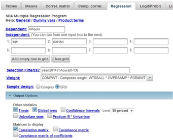
Figure 15-2

The first four boxes in your output are what you want to look at. 

• The first box lists the variables you entered as your dependent, independent, weight, and filter variables.
• The second box gives you the regression coefficients.
  • The unstandardized regression coefficient for age (B₁) is equal to 0.019 and the unstandardized regression coefficient for paeduc (B₂) is -0.083.  This means that an increase of one unit in paeduc results in an average decrease of -.083 units in tvhours after statistically adjusting for age.  Or, to put it another way, an increase of one year in the father’s education results in an average decrease of .083 hours of television viewing after statistically adjusting for the respondent’s age.  How would you interpret B₁?
  • So what does it mean to statistically adjust for something?  Suffice it to say that it means that B₁ tells us the effect or influence of X₁ on the dependent variable after taking into account the other independent variables (i.e., in this case X₂).   The other regression coefficient, B₂, would be similarly interpreted.
  • The regression constant is 2.700. This is referred to as the constant since it always stays the same regardless of which values of X₁ and X₂ you are using to predict Y.
  • The standard error of these coefficients which is an estimate of the amount of sampling error.
  • The standardized multiple regression coefficients (often referred to as Beta).  You can’t compare the unstandardized multiple regression coefficients (B₁ and B₂) because they have different units of measurement.  One year of age is not the same thing as one year of education.  The standardized multiple regression coefficients (Beta) are directly comparable.  You can see that the Beta for paeduc is -.184 and for age is .171 which means that father’s education is relatively more important in predicting hours of television viewing than is age. 
  • The t test which tests the null hypotheses that the population constant and population regression coefficients are equal to 0. 
  • The significance value for each test. As you can see in this example, we reject all three null hypotheses. However, we’re usually only interested in the t test for the regression coefficients. 
  • The value of the Multiple R and Multiple R-Squared.  The Multiple R squared tells us that age and paeduc together explain or account for 7.8% of the total variation in the number of hours per day that respondents watch television.   In the exercise STAT14S_SDA we saw that age by itself explained 3.8% of the variation in tvhours and that paeduc by itself explained 5.1%.  Why can’t we just add 3.8% and 5.1% and say that 8.9% of the total variation is explained by these two variables together.  We see from the SDA output that this is not true.  In fact, 7.8% of the total variation is explained by these two variables together.  Why is that?  It’s because the variation explained by these two independent variables overlap and because of this overlap they only account for 7.8% of the total variation in the dependent variable. 
  • The value of the Adjusted R-Squared which is 0.077.  The Adjusted R Square “takes into account the number of independent variables relative to the number of observations.” (George W. Bohrnstedt and David Knoke, Statistics for Social Data Analysis, 1994, F.E. Peacock, p. 293)

• The third box shows the Wald F-Statistic and its associated probability (P) which tests the null hypothesis that all the unstandardized and standardized regression coefficient are equal to 0.  Since the P value (.000) is less than .05 we can reject the null hypothesis and conclude that at least one coefficient is not 0.
• The fourth box shows the Pearson Correlation matrix for our three variables. As you can see, these correlations are similar for all three pairs of variables.

So our multiple regression equation for predicting Y is 2.700 + .019X₁ - .083X₂.  Thus for a person that is 20 years old and whose father completed 12 years of school,  the predicted number of hours that he or she watches television 2.700 + (.019) (20) - .083 (12) or 2.700 + 0.38 – 0.996 or 2.084 hours.

It’s important to keep in mind that everything we have done assumes that our dependent variable is a “linear function of more than one independent variable.”  (Colin Lewis-Beck and Michael Lewis-Beck, Applied Regression – An Introduction, Sage Publications, 2015, p. 55) 

Part III – It’s Your Turn Now

Use the same dependent variable, tvhours, but this time add educ to your list of independent variables.  Now you will have three independent variables – age, paeduc, and educ.  The variable educ is the years of school completed by the respondent.  Use SDA to get the regression equation.

• Write out the regression equation.
• What do the unstandardized multiple regression coefficients (B₁, B₂, and B₃) tell you?
• What do the standardized regression coefficients (Beta) tell you?
• What are the values of R and R² and what do they tell you?
• What are the different tests of significance that you can carry out and what do they tell you?

Part IV – Do we have a problem?

Multicollinearity occurs when the independent variables are highly correlated with each other.  If one of your independent variables is a perfect linear function of the other independent variables, then you would not be able to determine the regression coefficients.  But this is not typical.  What is more likely is that some of the independent variables might explain a large portion of the variation in another independent variable.  For example, in Part III what if both father’s education and age explained a very large portion of the variation in respondent’s education?  Then you would have high multicollinearity.  The problem that multicollinearity creates is that it tends to make your regression coefficients less reliable.  The standard errors of the regression coefficients increase which makes it harder to reject the null hypothesis in your t tests.

There are several ways to determine if multicollinearity is a problem in your analysis.  You can start by looking at the Pearson Correlation matrix for your independent variables.  Look at the correlation matrix in the SDA output to see if any of the independent variables are highly intercorrelated.   If they are, then you would have a problem but in this example it doesn’t appear this is the case.  There are other ways to detect multicollinearity but for this exercise we’ll stop here.