Author: Ed Nelson
Department of Sociology M/S SS97
California State University, Fresno
Fresno, CA 93740
Email: ednelson@csufresno.edu
Note to the Instructor: The data set used in this exercise is gss14_subset_for_classes_CONFIDENCE_SPENDING.sav which is a subset of the 2014 General Social Survey. Some of the variables in the GSS have been recoded to make them easier to use and some new variables have been created. The data have been weighted according to the instructions from the National Opinion Research Center. This exercise uses FREQUENCIES, CROSSTABS, and RECODE in SPSS to explore the relationship between confidence in the executive branch and whether respondents think we are spending too little, about right, or too much on the military and welfare. In this exercise we also control for political party identification. A good reference on using SPSS is SPSS for Windows Version 23.0 A Basic Tutorial by Linda Fiddler, John Korey, Edward Nelson (Editor), and Elizabeth Nelson. The online version of the book is on the The online version of the book is on the Social Science Research and Instructional Center's Website. You have permission to use this exercise and to revise it to fit your needs. Please send a copy of any revision to the author. Included with this exercise (as separate files) are more detailed notes to the instructors, the SPSS syntax necessary to carry out the exercise (SPSS syntax file), and the SPSS output for the exercise (SPSS output file). Pleas contact the author for additional information.
I'm attaching the following files.
- Data subset (.sav format).
- Extended notes for instructors (MS Word; .docx format).
- SPSS syntax file (.sps format).
- SPSS output file (.spv format).
- This page (MS Word; .docx format).
Goals of Exercise
The goal of this exercise is to determine whether confidence in the executive branch is related to whether respondents think we are spending too little, about right, or too much on the military and welfare with controls for political party identification. The exercise also gives you practice in using RECODE, FREQUENCIES and CROSSTABS in SPSS.
Part I—Choosing our Dependent Variable
We’re going to use the General Social Survey (GSS) for this exercise. The GSS is a national probability sample of adults in the United States conducted by the National Opinion Research Center (NORC). The GSS started in 1972 and has been an annual or biannual survey ever since. For this exercise we’re going to use a subset of the 2014 GSS. Your instructor will tell you how to access this data set which is called gss14_subset_for_classes_CONFIDENCE_SPENDING.sav.
There are a number of different areas or problems on which the government spends money. Some people think we should be spending more on some of these problems or areas while others think we should be spending less or about the same. The GSS uses the following question to measure spending priorities – “First I would like to talk with you about some things people think about today. We are faced with many problems in this country, none of which can be solved easily or inexpensively. I'm going to name some of these problems, and for each one I'd like you to tell me whether you think we're spending too much money on it, too little money, or about the right amount.” For this exercise were going to focus on whether respondents think we are spending too much, about right, or too little on the military (NAT3_NATARMS)[1] and welfare (NAT17_NATFARE).
These variables will be our dependent variables. Remember that the dependent variable is what we’re trying to explain. We want to explain why some people think we are spending too little on these issues while others think we are spending too much and still others feel we are spending about the right amount of money.
Part II – Choosing Our Independent Variable
Independent variables are variables that we think might explain why some people feel we are spending too little on the military and welfare while others think we are spending too much or about the right amount. There are many possible independent variables. We’re going to focus on the amount of confidence that respondents have in the executive branch of the federal government (CI5_CONFED).
We want to write a hypothesis that specifies the relationship that we expect to find between confidence in the executive branch and how respondents feel about spending on the military. Our hypothesis might be that the more confidence people have in the executive branch of the federal government, the more likely they are to think we are spending too much on the military and the less likely they are to feel we are spending too little.
Now we have a clear hypothesis that specifies the relationship we expect to find between confidence in the executive branch and spending priorities for the military. But why do we expect to find this relationship? We need to provide a clear and convincing argument to support our hypothesis. If we’re asked the why question, how will we respond? We might point out that it’s the president who is the commander-in-chief and who selects the Secretary of Defense (with the consent of Congress). In 2014 when the GSS was carried out, the President (Barack Obama) was a Democrat. In recent years the Republican Party has lobbied for more military spending while the Democratic Party tends to focus more on social spending. For these reasons those who have more confidence in the executive branch will feel that we ought to be spending less on the military and more on social issues.
Now it’s your turn. The other spending priority that we’re going to consider in this exercise is spending on welfare. Write a hypothesis that specifies the relationship that you expect to find between confidence in the executive branch (CI5_CONFED) and spending on welfare (NAT17_NATFARE). Then write an argument explaining why you expect to find this relationship.
Part III – Let’s Look at the Data
Now that we have a hypothesis and a rationale for our hypothesis, it’s time to look at the data. First, you need to be clear which is the dependent and independent variable. The dependent variable is what you are trying to explain which is why some people feel we are spending too much on the military and others think we are spending too much or about the right amount. The independent variable is the variable you think might help you explain differences of opinion on spending. In this case our hypothesis suggests that confidence in the executive branch influences spending priorities for the military.
Run CROSSTABS in SPSS to get the table that shows the relationship between these two variables (NAT3_NATARMS and CI5_CONFED). (See Crosstabulation in Chapter 5 of the SPSS online book.) Put the independent variable in the column and the dependent variables in the rows of your table. If you do this, you will always want to tell SPSS to compute the column percents. Also tell SPSS to compute Chi Square and an appropriate measure of association.
Here is the crosstabulation for the question that asks about spending on the military (NAT3_NATARMS).
To interpret the crosstabulation always compare the percents in the direction opposite to the way in which they sum to 100%. Since you asked for the column percents, the percents sum down to 100. That means that you want to compare the percents straight across. Look at the first row (i.e., too little). The more confidence people have in the executive branch, the less likely they are to feel that we are spending too little. On the other hand, the more confidence they have in the executive branch, the more likely they are to feel we’re spending too much. For example, 18.1% of those who have a great deal of confidence in the executive branch think we are spending too little on the military compared to 43.6% of those who have hardly any confidence. But 38.1% of those who have a great deal of confidence think we are spending too much on the military compared to 26.1% of those who had hardly any confidence.
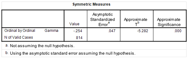
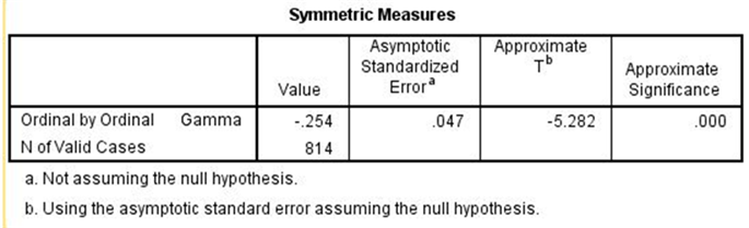
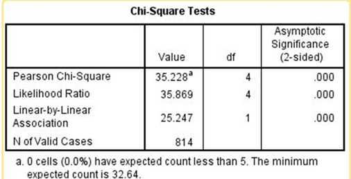
Chi Square is statistically significant and the Gamma value of -0.254 suggests a moderately strong relationship. Clearly the data support our hypothesis.
Part IV – Now It’s Your Turn
In Part 2, you wrote a hypothesis that specified the relationship that you expect to find between confidence in the executive branch (CI5_CONFED) and spending on welfare (NAT17_NATFARE). Now repeat the analysis that we carried out in Part 3 by telling SPSS to get the crosstabulation of CI5_CONFED and NAT17_NATFARE and write a paragraph describing the relationship between your two variables and whether the table supports your hypothesis. Be sure to tell SPSS to compute Chi Square and the appropriate measure of association. Use all this information to interpret the relationship between your two variables.
Part V – Bringing another Variable into the Analysis
There are other variables that are related to both confidence in the executive branch and spending on the military. One of those variables is political party identification (P1_PARTYID). Run a frequency distribution for this variable to see how it is coded.
We don’t want to use all seven categories for this variable so let’s recode P1_PARTYID by combining categories in the following way.
· Combine strong Democrat (value 0), not strong Democrat (value 1), and Independents, near Democrat (value 2) into once category. Give this category a value of 1 and call it “Democrat.”
· Leave Independent (value 3) as a separate category. Give this category a value of 2 and call it “Independent.”
· Combine Independent, near Republican (value 4), not strong Republican (value 5) and strong Republican (value 6) into another category. Give this category a value of 3 and call it “Republican.”
There are other ways we could combine the categories but let’s use this method. We’re going to use recoding into a different variable in SPSS. Give this new variable the name of P1_PARTYID1. To make your output easier to read, add variable and value labels for your new recoded variable. If you don’t know how to recode into another variable or how to add variable and value labels, your instructor will show you how. (See also Chapter 3 in the online SPSS book.)
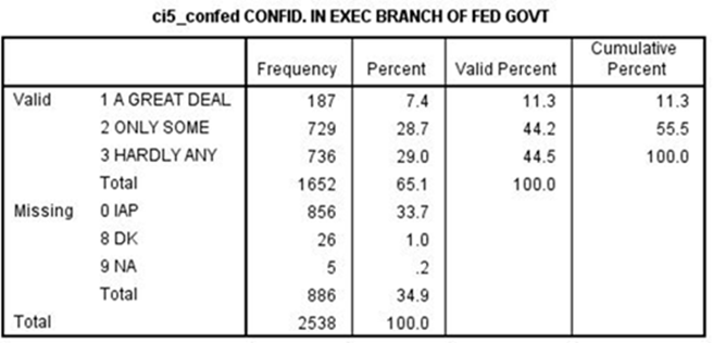
There is another variable that we also want to recode. Run a frequency distribution for CI5_CONFED.
Notice that there aren’t many respondents who have a great deal of confidence in the executive branch (i.e. only 11.3%). This is going to cause a problem later on. We’ll explain why later in this exercise. So let’s recode it now in the following way.
· Combine a great deal (value 1) and only some (value 2) into one category. Give this category a value of 1 and call it “some or more.”
· Leave hardly any (value 3) as a separate category. Give this category a value of 2 and call it “hardly any.”
Give this new variable the name of CI5_CONFED1. To make your output easier to read, add variable and value labels for your new recoded variable. If you don’t know how to recode into another variable or how to add variable and value labels, your instructor will show you how. (See also Chapter 3 in the online SPSS book.)
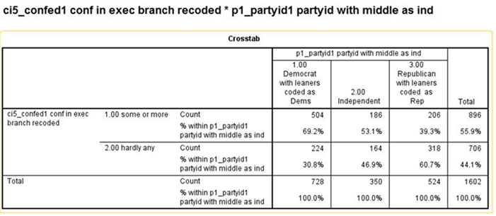
Now let’s make sure that party identification is related to both CI5_CONFED1 and NAT3_NATARMS. Tell SPSS to get the crosstabulation of P1_PARTYID1 with each of these variables. This will require that you run two crosstabulations. Use P1_PARTYID1 as your independent variable.
· P1_PARTYID1 and CI5_CONFED1
· P1_PARTYID1 and NAT3_NATARMS
Write a paragraph describing the relationship between P1_PARTYID1 and these two variables. Be sure to tell SPSS to compute Chi Square and the appropriate measure of association. Use all this information to interpret these two crosstabulations. Here are the tables that you should get from SPSS.[2]

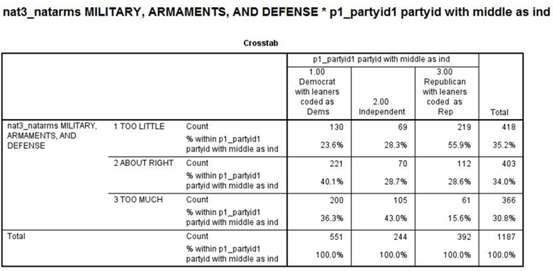
It’s clear from these tables that political party identification is related to both confidence and spending priorities for the military.
Part VI – Now It’s Your Turn Again
Now repeat the analysis that we carried out in Part V. Tell SPSS to get the crosstabulation of P1_PARTYID1 and NAT17_NATFARE and write a paragraph describing the relationship between your two variables. Be sure to tell SPSS to compute Chi Square and an appropriate measure of association. Use all this information to interpret the relationship between your two variables.
Part VII – Bringing Party Identification into the Analysis
Now that we know that political party identification is related to both confidence in the executive branch and spending priorities that raises another possibility. Perhaps the reason that those who have more confidence in the executive branch are more likely to feel that we’re spending too much on the military is that Democrats have more confidence in the executive branch and are more inclined to think that we’re spending too much on the military than do Republicans.
We can check on this by rerunning the crosstabulation of confidence in the executive branch and spending on the military controlling for party identification. In other words, we’re going to separate our sample into three groups – Democrats, Independents, and Republicans – and look at the relationship between CI5_CONFED1 and NAT3_NATARMS separately for each of these three groups. Here’s what our table will look like.
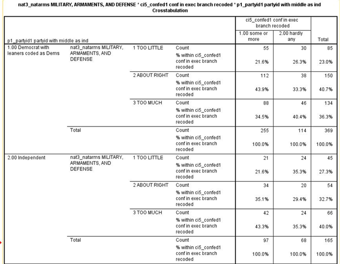
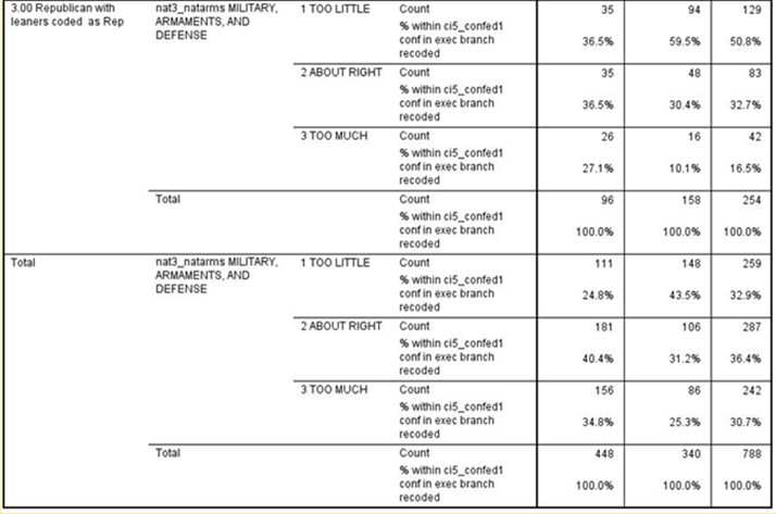
Note that we have four tables – one each for Democrats, Independents, and Republicans – and one for all three combined which SPSS calls total.
Here are the Chi Square and Gamma tables.
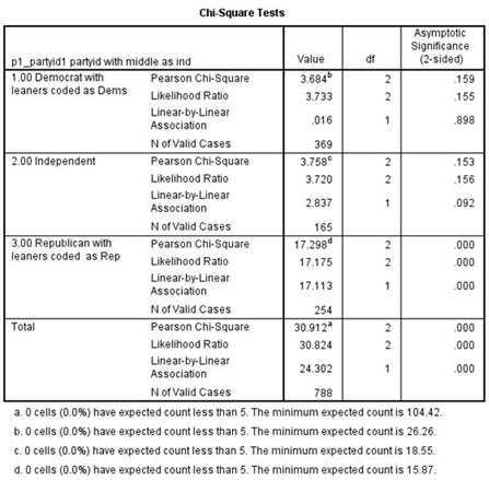
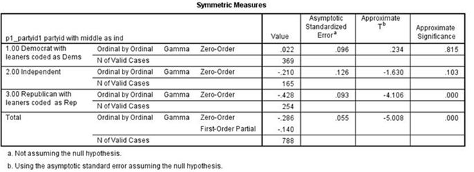
Note that again we have four tables -- one each for Democrats, Independents, and Republicans – and another for all three combined which SPSS calls total.[3]
If the relationship between confidence and spending priorities had been due to party identification, then the relationship would have disappeared or decreased markedly in each of the first three tables.[4] But what happened was that it decreased sharply for Democrats and Independents but not for Republicans. In other words, we discovered that the relationship exists primarily for Republicans but not for Democrats and Independents.[5]
Part VIII – Now It’s Your Turn Again
Now repeat this analysis that we carried out in Part VII but this time use NAT17_NATFARE as your dependent variable. Tell SPSS to get the crosstabulation of CI5_CONFED1 and NAT17_NATFARE controlling for P1_PARTYID1 and write a paragraph describing the relationship between these two variables when you control for political party identification. Be sure to tell SPSS to compute Chi Square and an appropriate measure of association. Use all this information to interpret the relationship between your two variables paying particular attention to what happened when you controlled for political party identification.
Part IX – Conclusions
Write a paragraph indicating what you learned about the relationship between confidence in the executive branch and spending priorities for welfare. Be as specific as possible.
[1] The names in all caps are the variable names.
[2] Note that I have omitted the Chi Square and Gamma tables for sake of brevity.
[3] Now we can explain why we recoded CI5_CONFED. Note that at the bottom of the Chi Square table, SPSS tells you the minimum expected frequency for each table. Chi Square assumes that this minimum expected frequency is at least 5 for each table. If we had not recoded CI5_CONFED we would have violated this assumption.
[4] This is often referred to as spuriousness.
[5] This is often referred to as specification.

