Author: Ed Nelson
Department of Sociology M/S SS97
California State University, Fresno
Fresno, CA 93740
Email: ednelson@csufresno.edu
Note to the Instructor: This exercise uses the 2014 General Social Survey (GSS) and SDA to explore Chi Square. SDA (Survey Documentation and Analysis) is an online statistical package written by the Survey Methods Program at UC Berkeley and is available without cost wherever one has an internet connection. The 2014 Cumulative Data File (1972 to 2014) is also available without cost by clicking here. For this exercise we will only be using the 2014 General Social Survey. A weight variable is automatically applied to the data set so it better represents the population from which the sample was selected. You have permission to use this exercise and to revise it to fit your needs. Please send a copy of any revision to the author. Included with this exercise (as separate files) are more detailed notes to the instructors and the exercise itself. Please contact the author for additional information.
I’m attaching the following files.
- Extended notes for instructors (MS Word; .docx format).
- This page (MS Word; .docx format).
Goals of Exercise
The goal of this exercise is to introduce Chi Square as a test of significance. The exercise also gives you practice in using CROSSTABS in SDA.
Part I—Relationships between Variables
We’re going to use the General Social Survey (GSS) for this exercise. The GSS is a national probability sample of adults in the United States conducted by the National Opinion Research Center (NORC). The GSS started in 1972 and has been an annual or biannual survey ever since. For this exercise we’re going to use the 2014 GSS. To access the GSS cumulative data file in SDA format click here. The cumulative data file contains all the data from each GSS survey conducted from 1972 through 2014. We want to use only the data that was collected in 2014. To select out the 2014 data, enter year(2014) in the Selection Filter(s) box. Your screen should look like Figure 10_1. This tells SDA to select out the 2014 data from the cumulative file.
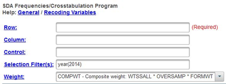
Figure 10-1
Notice that a weight variable has already been entered in the WEIGHT box. This will weight the data so the sample better represents the population from which the sample was selected.
The GSS is an example of a social survey. The investigators selected a sample from the population of all adults in the United States. This particular survey was conducted in 2014 and is a relatively large sample of approximately 2,500 adults. In a survey we ask respondents questions and use their answers as data for our analysis. The answers to these questions are used as measures of various concepts. In the language of survey research these measures are typically referred to as variables. Often we want to describe respondents in terms of social characteristics such as marital status, education, and age. These are all variables in the GSS.
In the previous exercise (STAT9S_SDA) we used crosstabulation and percents to describe the relationship between pairs of variables in the sample. But we want to go beyond just describing the sample. We want to use the sample data to make inferences about the population from which the sample was selected. Chi Square is a statistical test of significance that we can use to test hypotheses about the population. Chi Square is the appropriate test when your variables are nominal or ordinal (see exercise STAT1S_SDA).
Before we look at the relationship between variables, we need to talk about independent and dependent variables. The dependent variable is whatever you are trying to explain. We could be trying to explain how people feel about abortion. The independent variable is some variable that you think might help you explain why some people think abortion should be legal and others think it shouldn’t be legal. We’re going to use sex as our independent variable. Normally we put the dependent variable in the row and the independent variable in the column. We’ll follow that convention in this exercise.
Run CROSSTABS in SDA to produce the crosstabulation of abany and sex. Click on OUTPUT OPTIONS and look at PERCENTAGING. Since your independent variable is in the column, you want to use the column percents. By default, the box for column percents is already checked. Your screen should look like Figure 10-2. Notice that the SELECTION FILTER(S) box and the WEIGHT box are both filled in. Click on RUN THE TABLE to produce the crosstabulation.
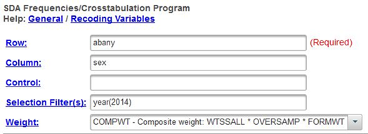
Figure 10-2
Part II – Interpreting the Percents
Your table should look like this.

Figure 10-3
Since your percents sum down to 100% (i.e., column percents), you want to compare the percents across. Look at the first row. Approximately 47% of men think abortion should be legal for any reason compared to 44% of women. This is a difference of 3.6% which seems rather small. We never want to make too much of small differences. Why not? No sample is ever a perfect representation of the population from which the sample is drawn. This is because every sample contains some amount of sampling error. Sampling error is inevitable. There is always some amount of sampling error present in every sample. The larger the sample size, the less the sampling error and the smaller the sample size, the more the sampling error.
But what is a small percent difference? Probably you would agree that a one to four percent difference is small. But what about a five or six or seven percent difference? Is that small? Or is it large enough for us to conclude that there is a difference between men and women in the population. Here’s where we can use Chi Square.
Part III – Chi Square
Let’s assume that you think that sex and opinion about abortion are related to each other. We’ll call this our research hypothesis. It’s what we expect to be true. But there is no way to prove the research hypothesis directly. So we’re going to use a method of indirect proof. We’re going to set up another hypothesis that says that the research hypothesis is not true and call this the null hypothesis. In our case, the null hypothesis would be that the two variables are unrelated to each other.[1] In statistical terms, we often say that the two variables are independent of each other. If we can reject the null hypothesis, then we have evidence to support the research hypothesis. If we can’t reject the null hypothesis, then we don’t have any evidence in support of the research hypothesis. You can see why this is called a method of indirect proof. We can’t prove the research hypothesis directly but if we can reject the null hypothesis then we have indirect evidence that supports the research hypothesis.
Here are our two hypotheses.
- research hypothesis – sex and opinion about abortion are related to each other
- null hypothesis – sex and opinion about abortion are unrelated to each other; in other words, they are independent of each other
It’s the null hypothesis that we are going to test.
SDA will compute Chi Square for you. Follow the same procedure you used to get the crosstabulation between sex and abany. Remember to get the column percents. Click on OUTPUT OPTIONS and then check the box for SUMMARY STATISTICS. Be sure to select SRS in the SAMPLE DESIGN line. Finally, click on RUN THE TABLE.
In the SUMMARY STATISTICS part of the output, you’ll see two Chi Squares – Chisq-P and Chisq-LR. We want to use the first one listed – Chisq-P. This is usually referred to as the Pearson Chi Square. The number in parentheses which in this case is 1 is the degrees of freedom.
The value of the Pearson Chi Square is 2.15. Your instructor may or may not want to go into the computation of the Chi Square value but we’re not going to cover it in this exercise.
The degrees of freedom (df) is 1. Degrees of freedom is number of values that are free to vary. In a table with two columns and two rows only one of the cell frequencies is free to vary assuming the marginal frequencies are fixed. The marginal frequencies are the values in the margins of the table. There are 766 males and 898 females in this table and there are 752 that think abortion should be legal for any reason and 912 who think abortion should not be legal for any reason. Try filling in any one of the cell frequencies in the table. The other three cell frequencies are then fixed assuming we keep the marginal frequencies the same.
Now we have to decide if we should reject the null hypothesis that the two variables are unrelated (or statistically independent) based on the Chi Square value and the degrees of freedom. Look at your output again and you’ll see that after the Chi Square value it says (p=0.14). That is the probability that you would be wrong if you rejected the null hypothesis. In other words, we would be wrong 14 out of 100 times. With odds like that, of course, we’re not going to reject the null hypothesis. A common rule is to reject the null hypothesis if the significance value is less than .05 or less than five out of one hundred. Since .14 is not smaller than .05, we don’t reject the null hypothesis. Since we can’t reject the null hypothesis, we don’t have any support for our research hypothesis.
Part IV – Now it’s Your Turn
Choose any two of the tables from the following list and compare men and women using crosstabulation and Chi Square.
- satisfaction with current financial situation (satfin)
- opinion about gun control (gunlaw)
- religiosity (reliten)
Make sure that you put the independent variable in the column and the dependent variable in the row. Be sure to ask for the correct percents and Chi Square. What are the research hypothesis and the null hypothesis? Do you reject the null hypothesis? How do you know? What does that tell you about the research hypothesis?
Part V – Expected Values
We said we weren’t going to talk about how you compute Chi Square but we do have to introduce the idea of expected values. The computation of Chi Square is based on comparing the observed cell frequencies (i.e., the cell frequencies that you see in the table that SDA gives you) and the cell frequencies that you would expect by chance assuming the null hypothesis was true. Your instructor may want to show you how to calculate the expected values by hand. We’re not going to go into it in this exercise.
Chi Square assumes that all the expected cell frequencies are greater than five. For the crosstabulation of abany and sex this is not a problem. All the expected frequencies are greater than five. If they are just a little bit below five, that’s no problem. But if they get down to around three you have a problem. What you’ll have to do is to combine rows or columns that have small marginal frequencies in order to increase the expected frequencies values.
Let’s look at an example where the expected frequencies are considerably less than five. Run the crosstabulation of sex and sibs which is the number of brothers and sisters that respondents have.[2] Some of the expected frequencies are so small that they are just about 0. That’s because there are aren't many respondents with more than 7 siblings. You will need to recode the number of siblings into fewer categories to increase the size of the expected frequencies.
We’ll recode sibs by combining all values from 8 through 25 into a single category and leaving the other categories the same. We can do this be entering the following in the ROW box – sibs(r:0=0;1=1;2=2;3=3;4=4;5=5;6=6;7=7;8=8-25 "8 or more") (Note: there is no period at the end of the command.)
Note the syntax for the recode statement since you will want to use it later.
- First you enter r: followed by the variable name which is sibs. The r stands for recode.
- Then you indicate the new value you want to assign to the recoded category.
- Then you put the old values that you are combining (or leaving as is). If there is a range of values that you are combining, then these values must be separated by a dash (i.e., hyphen).
- This is followed by the label you want to assign to the new category enclosed in double quotation marks which is “8 or more” for the category 8. This is optional and is free form meaning you can put what you want for the label.
- Recoded categories are separated by a semi-colon.
- Finally, the entire recode specification is in parentheses.
- So your recode statement looks like this: sibs(r:0=0;1=1;2=2;3=3;4=4;5=5;6=6;7=7;8=8-25 "8 or more")
Enter this into the ROW box and then click on RUN THE TABLE to rerun the crosstab using the recoded sibs. Now your expected frequencies will be large enough to meet the assumption that all expected values are greater than 5. Compare the value of Chi Square for the unrecoded sibs with the recoded sibs. Are they the same? Why or why not?
[1] The null hypothesis is often called the hypothesis of no difference. We’re saying that there is no relationship between these two variables. In other words, there’s nothing there.
[2] Number of siblings is a ratio level variable. You can use Chi Square with ratio level variables but usually there are better tests. We’re just using this as an example.

