Author: Ed Nelson
Department of Sociology M/S SS97
California State University, Fresno
Fresno, CA 93740
Email: ednelson@csufresno.edu
Note to the Instructor: This exercise uses the 2014 General Social Survey (GSS) and SDA to explore levels of measurement. SDA (Survey Documentation and Analysis) is an online statistical package written by the Survey Methods Program at UC Berkeley and is available without cost wherever one has an internet connection. The 2014 Cumulative Data File (1972 to 2014) is also available without cost by clicking here. For this exercise we will only be using the 2014 General Social Survey. A weight variable is automatically applied to the data set so it better represents the population from which the sample was selected. You have permission to use this exercise and to revise it to fit your needs. Please send a copy of any revision to the author. Included with this exercise (as separate files) are more detailed notes to the instructors and the exercise itself. Please contact the author for additional information.
I’m attaching the following files.
- Extended notes for instructors (MS Word; .docx format).
- This page (MS Word; .docx format).
Goals of Exercise
The goal of this exercise is to explore the concept of levels of measurement (nominal, ordinal, interval, and ratio measures) which is an important consideration for the use of statistics. The exercise also gives you practice in using FREQUENCIES in SDA.
Part I—Introduction to Levels of Measurement
We use concepts all the time. We all know what a book is. But when we use the word “book” often we’re not talking about a particular book that we’re reading. We’re talking about books in general. In other words, we’re talking about the concept to which we have given the name “book.” There are many different types of books – paperback, hardback, small, large, short, long, and so on. But they all have one thing in common – they all belong to the category “book.”
Let’s look at another example. Religiosity is a concept which refers to the degree of attachment that individuals have to their religious preference. It’s different than religious preference which refers to the religion with which they identify. Some people say they are Lutheran; others say they are Roman Catholic; still others say they are Muslim; and others say they have no religious preference. Religiosity and religious preference are both concepts.
A concept is an abstract idea. So there are the abstract ideas of book, religiosity, religious preference, and many others. Since concepts are abstract ideas and not directly observable, we select measures or indicants of these concepts. Religiosity can be measured in a number of different ways – how often people attend church, how often they pray, and how important they say their religion is to them.
We’re going to use the General Social Survey (GSS) for this exercise. The GSS is a national probability sample of adults in the United States conducted by the National Opinion Research Center (NORC). The GSS started in 1972 and has been an annual or biannual survey ever since. For this exercise we’re going to use the 2014 GSS. To access the GSS cumulative data file in SDA format click here. The cumulative data file contains all the data from each GSS survey conducted from 1972 through 2014. We want to use only the data that was collected in 2014. To select out the 2014 data, enter year(2014) in the Selection Filter(s) box. Your screen should look like Figure 1-1. This tells SDA to select out the 2014 data from the cumulative file.
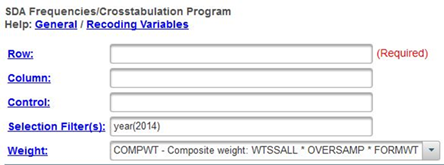
Figure 1-1
Notice that a weight variable has already been entered in the WEIGHT box. This will weight the data so the sample better represents the population from which the sample was selected.
The GSS is an example of a social survey. The investigators selected a sample from the population of all adults in the United States. This particular survey was conducted in 2014 and is a relatively large sample of approximately 2,500 adults. In a survey we ask respondents questions and use their answers as data for our analysis. The answers to these questions are used as measures of various concepts. In the language of survey research these measures are typically referred to as variables. Often we want to describe respondents in terms of social characteristics such as marital status, education, and age. These are all variables in the GSS.
These measures are often classified in terms of their levels of measurement. S. S. Stevens described measures as falling into one of four categories – nominal, ordinal, interval, or ratio.[1]
Here’s a brief description of each level.
A nominal measure is one in which objects (i.e. in our survey, these would be the respondents) are sorted into a set of categories which are qualitatively different from each other. For example, we could classify individuals by their marital status. Individuals could be married or widowed or divorced or separated or never married. Our categories should be mutually exclusive and exhaustive. Mutually exclusive means that every individual can be sorted into one and only one category. Exhaustive means that every individual can be sorted into a category. We wouldn’t want to use single as one of our categories because some people who are single can also be divorced and therefore could be sorted into more than one category. We wouldn’t want to leave widowed off our list of categories because then we wouldn’t have any place to sort these individuals.
The categories in a nominal level measure have no inherent order to them. This means that it wouldn’t matter how we ordered the categories. They could be arranged in any number of different ways. Run FREQUENCIES in SDA for the variable marital so you can see the frequency distribution for a nominal level variable. It wouldn’t matter how we ordered these categories. To run the frequency distribution, enter the variable name, marital, in the ROW box. Your screen should like Figure 1-2. Then click on RUN THE TABLE at the bottom. Notice that the SELECTION FILTER(S) box and the WEIGHT box are both filled in.
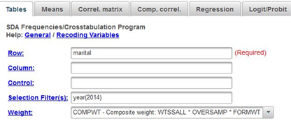
Figure 1-2
An ordinal measure is a nominal measure in which the categories are ordered from low to high or from high to low. We could classify individuals in terms of the highest educational degree they achieved. Some individuals did not complete high school; others graduated from high school but didn’t go on to college. Other individuals completed a two-year junior college degree but then stopped college. Still others completed their bachelor’s degree and others went on to graduate work and completed a master’s degree or their doctorate. These categories are ordered from low to high.
But notice that while the categories are ordered they lack an equal unit of measurement. That means, for example, that the differences between categories are not necessarily equal. Run FREQUENCIES in SDA for degree. Look at the categories. The GSS assigned values (i.e., numbers) to these categories in the following way:
- 0 = less than high school,
- 1 = high school degree,
- 2 = junior college,
- 3 = bachelors, and
- 4 = graduate.
The difference in education between the first two categories is not the same as the difference between the last two categories. We might think they are because 0 minus 1 is equal to 3 minus 4 but this is misleading. These aren’t really numbers. They’re just symbols that we have used to represent these categories. We could just as well have labeled them a, b, c, d, and e. They don’t have the properties of real numbers. They can’t be added, subtracted, multiplied, and divided. All we can say is that b is greater than a and that c is greater than b and so on.
An interval measure is an ordinal measure with equal units of measurement. For example, consider temperature measured in degrees Fahrenheit. Now we have equal units of measurement – degrees Fahrenheit. The difference between 20 degrees and 40 degrees is the same as the difference between 70 degrees and 90 degrees. Now the numbers have the properties of real numbers and we can add them and subtract them. But notice one thing about the Fahrenheit scale. There is no absolute zero point. There can be both positive and negative temperatures. That means that we can’t compare values by taking their ratios. For example, we can’t divide 80 degrees Fahrenheit by 40 degrees and conclude that 80 is twice as hot at 40. To do that we would need a measure with an absolute zero point.[2]
A ratio measure is an interval measure with an absolute zero point. Run FREQUENCIES for sibs which is the number of siblings. This variable has an absolute zero point and all the properties of nominal, ordinal, and interval measures and therefore is a ratio variable.
Notice that level of measurement is itself ordinal since it is ordered from low (nominal) to high (ratio). It’s what we call a cumulative scale. Each level of measurement adds something to the previous level.
Why is level of measurement important? One of the things that helps us decide which statistic to use is the level of measurement of the variable(s) involved. For example, we might want to describe the central tendency of a distribution. If the variable was nominal, we would use the mode. If it was ordinal, we could use the mode or the median. If it was interval or ratio, we could use the mode or median or mean. Central tendency will be the focus of another exercise (STAT2S_SDA).
Run FREQUENCIES for the following variables:
- satfin,
- wealth.
- happy,
- partyid,
- relig,
- denom,
- reliten,
- nummen,
- numwomen,
- premarsx, and
- age.
For each variable, decide which level of measurement it represents and write a sentence or two indicating why you think it is that level. Keep in mind that we’re only considering those responses that answered the question asked of the respondent. Not all respondents answered the question. Some said they didn’t know or refused to answer the question. These respondents are assigned missing values to indicate they didn’t answer the question and are not included in the frequency distribution.
[1] Stanley Smith Stevens, 1946, “On the Theory of Scales of Measurement,” Science 103 (2684), pp. 677-680.
[2] You might wonder why we didn’t use an example from the GSS. There isn’t one. They don’t occur in social science research very often. There are examples from the field of business. Think about profit for businesses over a fiscal year. There is no absolute zero. Profit could be positive or negative.

